Frequency-Resolved Analysis
The fitted transfer function can be partitioned into smooth frequency bands and transformed back to the lag domain. This gives a time-frequency style view of the recovered kernel instead of a single kernel collapsed across the whole fitted spectrum.
Frequency-Resolved Weights
resolved = model.frequency_resolved_weights(
    n_bands=18,
    fmax=min(100.0, float(model.frequencies[-1])),
    value_mode="real",
)

fig, ax = model.plot_frequency_resolved_weights(
    resolved=resolved,
    input_index=0,
    output_index=0,
)
This produces a frequency-by-lag map for one input/output pair while leaving
the ordinary kernel available in model.weights.
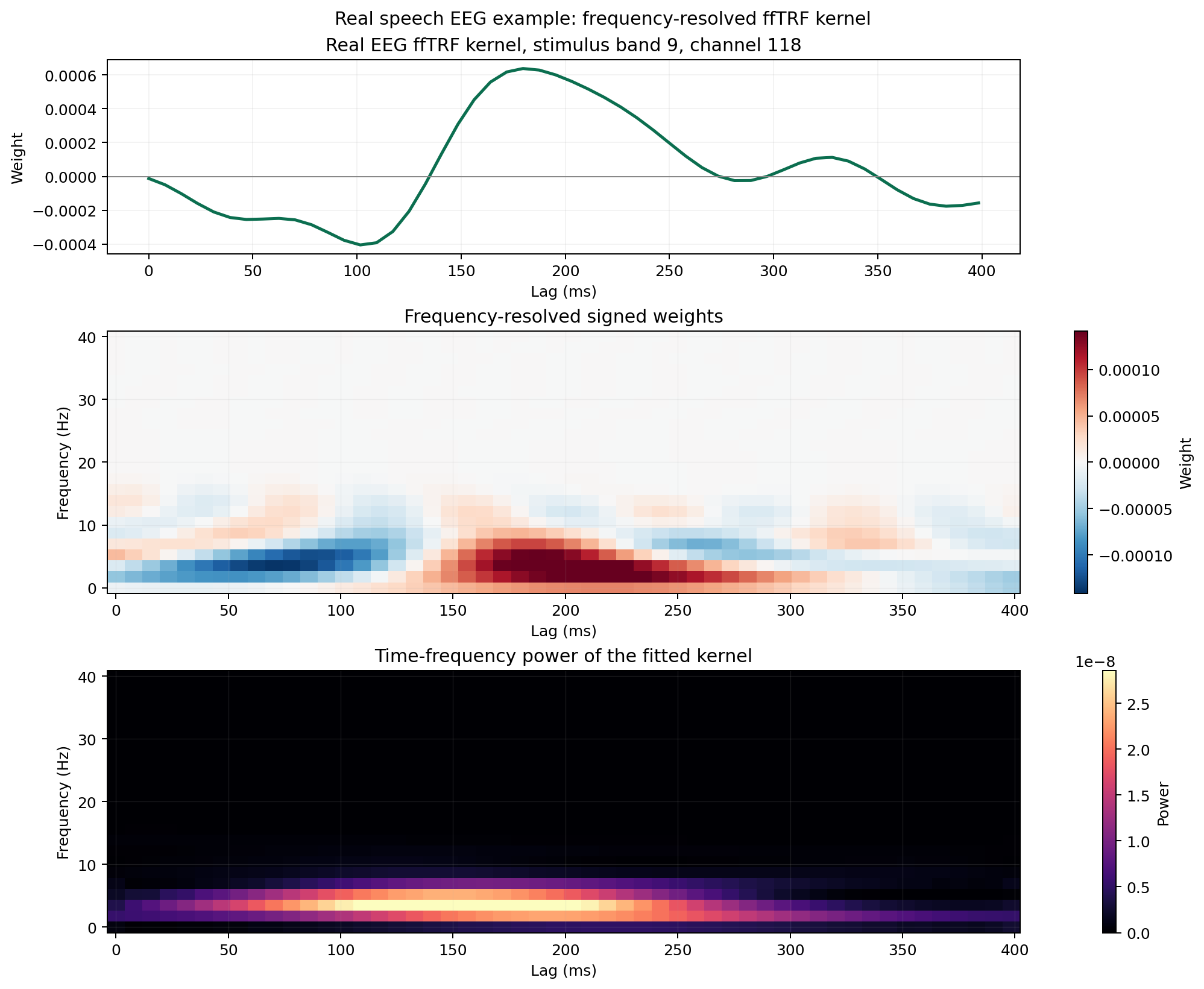
In the real speech EEG example, this view highlights which lag/frequency regions of a fitted forward kernel carry most structure:
What the Parameters Mean
n_bands: number of analysis bandsfmin,fmax: frequency range to resolve;fmaxmust stay at or below the fitted Nyquist frequency (fs / 2)scale:"linear"or"log"spacing of band centersbandwidth: width of the Gaussian analysis bandsvalue_mode: how the band-limited kernels are represented
Choosing value_mode
value_mode="real"keeps signed band-limited kernelsvalue_mode="magnitude"takes their absolute valuevalue_mode="power"squares the magnitude
Use real when you care about polarity and cancellation across lags. Use
magnitude or power when you want a simpler non-negative map.
Time-Frequency Power
power = model.time_frequency_power(
    n_bands=18,
    method="hilbert",
)

fig, ax = model.plot_time_frequency_power(
    power=power,
    input_index=0,
    output_index=0,
)
This view starts from the signed band-limited kernels and turns each band into a smoother positive power estimate using the analytic-signal magnitude.
When to Use Which View
- Use
frequency_resolved_weights(..., value_mode="real")when you want signed structure in the recovered kernel. - Use
frequency_resolved_weights(..., value_mode="magnitude")when you want a simpler non-negative map without the extra Hilbert step. - Use
time_frequency_power(...)when you want a spectrogram-like summary of kernel energy.
Interpretation Tips
- These plots describe the fitted kernel, not the raw stimulus or response.
- Summing across the band axis in the default signed view approximates the ordinary lag-domain kernel.
- Log-spaced bands are often more interpretable when you care about a broad range of frequencies.
Diagnostics Around the Transfer Function
The estimator also exposes direct frequency-domain views:
transfer_function_at(...)transfer_function_components_at(...)plot_transfer_function(...)cross_spectral_diagnostics(...)plot_coherence(...)plot_cross_spectrum(...)
If you want the same workflow in a more tutorial-like format, see the rendered Frequency-Resolved Notebook.